Table of Contents
- Why I keep worrying about qubit overhead
- Stabilizer codes and the surface code, in one sitting
- The locality tax: a hard bound in two dimensions
- qLDPC codes and the wiring problem
- Tile codes: surface codes that come in shapes
- The iSWAP idea: turning a gate into a conveyor belt
- Directional tile codes: the 2026 synthesis
- A worked example I can draw by hand
- How good are they, in numbers
- The punchline in one table
- Caveats, and what I am watching next
- Conclusion
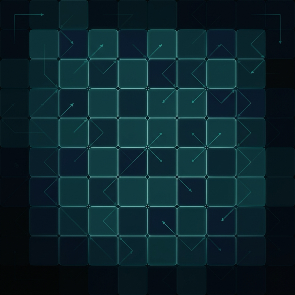
Visualizing directional measurement walks across a square qubit grid, where check qubits trace compass-step paths to collect stabilizer parity via nearest-neighbour gates.
Why I keep worrying about qubit overhead
Let me set the scene with a number that bothers me. Suppose I want a single protected logical qubit using the most popular code on superconducting hardware, the rotated surface code. If I want it to survive errors of distance \(d\), I pay roughly \(2 d^2\) physical qubits for that one logical qubit. At distance \(15\) that is around \(450\) physical qubits doing the work of one. If my eventual algorithm needs a thousand logical qubits, the bookkeeping becomes painful very quickly.
The dream alternative is a family called quantum low density parity check codes, written qLDPC, which can pack many logical qubits into one block while keeping every parity check small. The catch, and the reason I am writing this post, is that the most powerful qLDPC codes ask for wiring that simply does not fit on a flat chip. So the practical question I care about is sharp: can I get the storage efficiency of qLDPC codes without giving up the friendly square grid that makes the surface code buildable today? The recent answer is yes, and the construction that gets there is the directional tile code.
Stabilizer codes and the surface code, in one sitting
A stabilizer code is defined by a set of commuting Pauli operators \(S_1, S_2, \dots\) called stabilizers. The protected states are exactly the ones that every stabilizer leaves untouched,
Measuring a stabilizer does not disturb a valid codeword, but if an error has occurred, some stabilizers flip their measured value from \(+1\) to \(-1\). That pattern of flips is the syndrome, and a decoder reads it like a detective reading footprints to infer which error happened and how to undo it.
The surface code is the friendliest concrete example. Picture a square lattice. I place a physical data qubit on every edge. At every vertex I define a star operator, and on every face I define a plaquette operator,
which on the bulk lattice are simply \(X \otimes X \otimes X \otimes X\) and \(Z \otimes Z \otimes Z \otimes Z\) acting on four neighbouring edges. Every check involves only qubits that sit right next to each other, which is the whole reason the surface code is so hardware friendly: nearest neighbour couplers are enough.
I summarise a code by three numbers, the parameters \([[n,k,d]]\): \(n\) physical qubits, \(k\) logical qubits, and distance \(d\), the size of the smallest error that can corrupt the encoded information without being caught. Bigger \(k\) is more storage, bigger \(d\) is more protection, and smaller \(n\) is less hardware. A rotated surface code patch is \([[d^2, 1, d]]\). One logical qubit. That single number \(k=1\) is the source of all my complaints.
A useful way to keep score across codes is the code efficiency ratio
which equals exactly \(1\) for a rotated surface code patch, since \(k d^2 / n = 1 \cdot d^2 / d^2 = 1\). Anything with \(\eta\) comfortably above \(1\) is doing better than the surface code at the same distance, packing more protected qubits into the same silicon.
The locality tax: a hard bound in two dimensions
Here is the theorem that frames everything that follows. If I insist that all my stabilizer checks are geometrically local on a two dimensional lattice, meaning each check only touches qubits within a bounded patch, then nature charges a tax. Bravyi, Poulin and Terhal proved that such codes must obey
so the code efficiency ratio \(\eta = k d^2 / n\) cannot keep growing without bound as the code gets large [2]. In plain words, in strictly local two dimensional layouts you cannot have high rate and large distance at the same time once the block gets very big.
I want to flag the precise loophole right now, because the recent work lives inside it. The bound is an asymptotic statement about the large block limit. It says nothing about the finite sizes that matter for the first generation of fault tolerant machines. At a fixed, buildable size, \(\eta\) of eight or ten is perfectly allowed, and that is exactly the regime where the surface code is wasteful and where a better code pays off. So the right target is not to beat an asymptotic bound, which is impossible, but to win convincingly at realistic finite sizes.
qLDPC codes and the wiring problem
So how do people escape \(k = 1\)? They give up strict two dimensional locality. Quantum low density parity check codes keep every check small, which is the low density part, but they let the checks reach across the chip. A celebrated example is the bivariate bicycle family, including the \([[144, 12, 12]]\) code nicknamed the gross code, which protects twelve logical qubits with weight six checks [3]. On paper this is a huge improvement in efficiency over twelve separate surface code patches.
The price is connectivity. Some of those weight six checks join qubits that are nowhere near each other on a flat layout. To realise them, hardware designers reach for long range couplers, vertical routing through stacked chips, or physically moving qubits around, all of which add real engineering difficulty. This is the wall I kept running into: marvelous codes that the chip cannot easily wire. The tile code program is, in my reading, a sustained attempt to climb over this wall while keeping both feet on a flat grid.
Tile codes: surface codes that come in shapes
The first big step is the tile code, introduced in 2025 [4]. The idea is delightfully geometric. A surface code uses two fixed shapes, the four qubit star and the four qubit plaquette, repeated everywhere. A tile code says: why fix the shape? Let me choose a more interesting tile, a small connected pattern of qubits, and use that as my repeating stabilizer instead.
Concretely, I work on a \(B \times B\) square grid and put data qubits on the edges. A tile is just a chosen subset of those edges, and it tells me the support of one stabilizer check. I lay an \(X\) type tile pattern and a \(Z\) type tile pattern across the grid, with translation invariant checks in the bulk and slightly trimmed checks at the boundary, exactly like a surface code has a clean interior and special edges.
The one rule I must respect is that \(X\) checks and \(Z\) checks have to commute. For tiles this becomes a clean combinatorial condition. Roughly, for every edge that the \(X\) tile occupies at some position, the \(Z\) tile must occupy the matching complementary edge at the mirrored position, so that the two shapes always overlap in an even number of places. When that mutual condition holds, the whole construction is a valid Calderbank, Shor and Steane (CSS) code by design.
The payoff is real. By searching over tile shapes, the authors found planar codes that crush the surface code on efficiency. A few highlights are collected below.
| Code \([[n,k,d]]\) | Check weight | \(\eta = k d^2 / n\) | Comment |
|---|---|---|---|
| \([[288, 8, 12]]\) | 6 | \(4.0\) | planar, bounded reach |
| \([[288, 8, 14]]\) | 8 | \(5.4\) | higher distance |
| \([[512, 18, 19]]\) | 8 | \(12.7\) | beats surface code by more than 12 times |
There is one honest caveat about the 2025 version. Some of those handsome tiles still require check to data couplings that are not strictly nearest neighbour; the reach is bounded but not always to the very next qubit. So tile codes solved the planarity and efficiency problem, yet a small connectivity gap remained between the code on paper and the gates a plain grid actually offers. Closing that last gap is what the newest work does.
The iSWAP idea: turning a gate into a conveyor belt
The trick that closes the gap is a change in how I think about a particular two qubit gate. On superconducting chips the iSWAP gate is native, and as the name suggests it swaps the states of two neighbouring qubits, up to phases. Normally I would treat a swap as a nuisance, just shuffling data around. The directional codes of 2025 reframed it as a feature [5]: if a check qubit swaps its way along a line of data qubits, then at each step it sits next to a fresh data qubit and can entangle with it.
Here is the analogy I find accurate and helpful. Imagine a clerk walking down a row of desks. At each desk the clerk both collects a signature (the parity information) and then steps to the next desk (the swap). By the time the clerk reaches the end of the row, the running tally on the clerk's clipboard equals the parity of the whole row, and crucially the clerk only ever talked to the person immediately in front of them. The iSWAP gate plays both roles at once: it is the entangling handshake and the step forward, fused into a single nearest neighbour operation.
This means a check that, drawn statically, looks nonlocal can instead be measured dynamically as a short walk across the grid. The nonlocality is moved out of the wiring diagram and into time. That single shift is the engine of the newest result.
Directional tile codes: the 2026 synthesis
The directional tile code, introduced in June 2026 under the title that nearest neighbour gates are all you need, marries the two ideas above [6]. From the tile codes it takes planar open boundary layouts with excellent finite size parameters. From the directional codes it takes the iSWAP walk. The bridge between them is a small object called a directional word.
A directional word is an ordered string of compass steps,
This one little string wears three hats at once, which is the part I find elegant:
- Geometry. Traced out on the grid, the word draws a bounded connected string of edges. That string is the shape of the tile.
- Algebra. Placing the same string on the primal lattice gives the \(X\) check, and placing it on the dual lattice gives the matching \(Z\) check, so one word fixes a valid commuting CSS pair.
- Schedule. The order of the steps is literally the order in which a check qubit walks through its data qubits during measurement.
So a single directional word simultaneously defines the code and the circuit that reads it. The weight of the word, \(w\), is the weight of the stabilizer.
The measurement walk and the CXSWAP gate
To make the walk concrete I need the exact gate. The paper expresses each data to check interaction as a CXSWAP, which is locally equivalent to an iSWAP up to single qubit Clifford rotations,
I like to read the right hand side as two jobs in one box. The \(\mathrm{CX}\) factor accumulates the stabilizer parity onto the check qubit, the signature collected at the desk. The \(\mathrm{SWAP}\) factor advances the qubits, the step to the next desk. For \(X\) checks the check qubit is the control; for \(Z\) checks the orientation is reversed after the usual basis change.
Where the walk would otherwise have to jump over an empty site, the layout inserts a routing qubit. A routing qubit prepared in \(\ket{0}\) lets the same gate act as a pure swap,
so routing and parity collection are compiled into one and the same nearest neighbour gate family. Nothing in the circuit ever reaches beyond an adjacent qubit.
One round, as pseudocode
Putting it together, a single round of syndrome extraction is the following walk. I have rewritten it in my own words from the paper's algorithm so the logic is easy to follow.
Input : directional word D = d_1 d_2 ... d_w, with each d_i in {N,E,S,W}
        a square grid holding data qubits, X checks, Z checks, routing qubits
Output: one round of syndrome extraction using only nearest neighbour gates

 1. Prepare every X check in |+> and every Z check in |0>.
 2. For i = 1 to w:
       For each check qubit q:
            let p = the neighbour of q in direction d_i
            if p is a data qubit:
                 if q is an X check : apply CXSWAP(q, p)
                 else               : apply CXSWAP(p, q)
            else if p is a routing qubit:
                 apply SWAP(q, p)
       For each routing qubit r:
            let p = the neighbour of r in direction d_i
            if p is a data qubit : apply SWAP(r, p)
 3. Measure every X check in the X basis and every Z check in the Z basis.

 Next round: run the reversed word. This returns every qubit to its start
 position and swaps the data and check roles, which flushes leakage out.
Two consequences of this structure are worth dwelling on.
Constant depth. For a word of weight \(w\), one round has depth \(w + 2\), counting the preparation and the measurement. That number depends only on the shape of the tile, never on how large the whole code is. So a giant directional tile code measures its checks just as fast as a tiny one, much as tying one shoelace does not take longer just because the closet holds more shoes, provided each is tied in parallel.
Free leakage cleanup. Real superconducting qubits sometimes leak into states outside the computational \(\{\ket{0}, \ket{1}\}\) space, and that leakage is a notorious headache. Because consecutive rounds run the word and then its reverse, the data and check qubits trade places every round. Both roles therefore get reset on a regular cadence, which sweeps accumulated population out of those higher states. The error correction and the leakage hygiene come from the very same swap dynamics, for free.
A worked example I can draw by hand
Abstract words deserve a picture. Take the short directional word
Starting from a corner and following the compass steps, the pen traces a little zigzag of five edges. I label the data qubits it crosses A, B, C, D, E in the order the walk meets them. In the diagram below, the letter o marks a lattice vertex, a double bar marks a horizontal edge, a single bar marks a vertical edge, and the capital letters sit on the edges that carry data qubits.
        o ==B== o          o
        |       |          |
        A       C          E
        |       |          |
        o       o ==D== o

   walk : start at lower left vertex
          N through A  ->  E through B  ->  S through C
          ->  E through D  ->  N through E  ->  finish
The \(X\) type tile is this exact string laid on the lattice; the \(Z\) type tile is the same string laid on the dual lattice, sitting so the two always overlap evenly and therefore commute. During measurement, one check qubit enters at the start and performs a CXSWAP at A, then B, then C, then D, then E, walking the path and collecting the parity \(X_A X_B X_C X_D X_E\) (or the corresponding \(Z\) string) onto itself, talking only to the qubit in front of it at every step. That is the entire idea, shrunk to something I can sketch on a napkin. The same word, applied as a tessellation rule on a finite patch, generates a genuine code; the smallest instances built from related words land at parameters like \([[18, 2, 3]]\) and \([[60, 4, 5]]\).
How good are they, in numbers
Now the part that made me sit up. The table below lists representative directional tile codes from the 2026 paper. Two scores appear. The code efficiency ratio \(\eta = k d^2 / n\) measures the underlying code, and the circuit efficiency ratio
measures the honest implemented layout, where \(n_{\mathrm{circ}}\) counts every physical qubit actually used, including data, check, and routing qubits, and \(n_{\mathrm{RSC}}(d)\) is the qubit count of one rotated surface code patch of the same distance. The final column is the simulated logical error rate per round per logical qubit at a physical error rate of \(0.001\).
| Directional word \(\Dword\) | \(w\) | \([[n,k,d]]\) | \(\eta = \tfrac{k d^2}{n}\) | \(\eta_{\mathrm{circ}}\) | \(p_L\) at \(p=0.001\) |
|---|---|---|---|---|---|
| \(\mathrm{N}^2\mathrm{E}\,\mathrm{S}\,\mathrm{E}\,\mathrm{N}^2\) | 7 | \([[60, 4, 5]]\) | \(1.67\) | \(1.34\) | \(7.8 \times 10^{-6}\) |
| \(\mathrm{N}^2\mathrm{E}\,\mathrm{S}\,\mathrm{E}\,\mathrm{N}^2\) | 7 | \([[180, 4, 9]]\) | \(1.80\) | \(1.59\) | \(1.5 \times 10^{-7}\) |
| \(\mathrm{N}^2\mathrm{E}^2\mathrm{S}\,\mathrm{E}^2\mathrm{N}^2\) | 9 | \([[217, 10, 7]]\) | \(2.26\) | \(1.74\) | \(2.2 \times 10^{-7}\) |
| \(\mathrm{N}^2\mathrm{E}^2\mathrm{S}\,\mathrm{E}\,\mathrm{S}\,\mathrm{E}^2\mathrm{N}^2\) | 11 | \([[182, 14, 10]]\) | \(7.69\) | \(5.84\) | \(4.3 \times 10^{-7}\) |
| \(\mathrm{N}^2\mathrm{E}^2\mathrm{S}\,\mathrm{E}\,\mathrm{S}\,\mathrm{E}^2\mathrm{N}^2\) | 11 | \([[323, 14, 15]]\) | \(9.75\) | \(7.89\) | dash |
| \(\mathrm{N}^2\mathrm{E}^2\mathrm{S}\,\mathrm{E}^3\mathrm{S}\,\mathrm{E}^2\mathrm{N}^2\) | 13 | \([[248, 20, 11]]\) | \(9.76\) | \(7.37\) | \(1.8 \times 10^{-7}\) |
The flagship is the \([[323, 14, 15]]\) code. Its code efficiency ratio is
nearly an order of magnitude above the surface code at the same distance. And the win is not just on paper: even after I add in the routing qubits that the nearest neighbour walk needs, the implemented circuit efficiency stays around \(7.9\). The headline claim from the simulations is that, at a footprint of roughly thirty circuit qubits per logical qubit and a physical error rate of \(0.001\), the best directional tile code layouts cut the logical error rate per round per logical qubit by up to a factor of about \(1000\) relative to rotated surface code memories storing the same number of logical qubits. Three orders of magnitude, on a square grid, with native gates.
The punchline in one table
The cleanest way I can summarise the whole arc is to ask three yes or no questions of each code family. Does it run with nearest neighbour gates on a square grid? Does it lay out as a flat patch with open boundaries? And does it reach an efficiency well above the surface code? Until now, every family answered no to at least one of them. The directional tile code is the first I know of that answers yes to all three.
| Code family | Nearest neighbour, square grid | Planar, open boundary | Efficiency well above surface code |
|---|---|---|---|
| Rotated surface code | yes | yes | no |
| qLDPC (gross code) | no | no | yes |
| Tile code (2025) | no | yes | yes |
| Toric directional code (2025) | yes | no | yes |
| Directional tile code (2026) | yes | yes | yes |
Caveats, and what I am watching next
I want to stay honest, because excitement is not a proof. A few things keep my expectations grounded.
First, the asymptotic bound from the earlier section has not been broken and never will be. The advantage here is a finite size advantage, exactly the kind the bound permits. That is the right thing to chase for early machines, but it is not a claim about arbitrarily large codes, and I would be wary of anyone who summarised it that way.
Second, the impressive logical error rates come from circuit level simulations under a uniform noise model at a physical error rate of \(0.001\). That is a standard and reasonable benchmark, yet real chips have correlated noise, crosstalk, and leakage that no single number fully captures. The construction is built to be leakage friendly through its role swapping, which is encouraging, but the paper is careful to note that it does not actually model leakage in its simulations, so that benefit is argued rather than measured.
Third, a memory is only half of a computer. Storing logical qubits efficiently is wonderful, but I eventually need fast, fault tolerant logical gates and a decoder that keeps up with the syndrome stream in real time. Understanding the logical operators and symmetries of tile codes is itself an active topic right now, and how cleanly directional tile codes support lattice surgery or other logical operations on the same grid is, in my view, the most important open question for turning this memory into computation.
Conclusion
What I take away is a small but satisfying lesson about where nonlocality can hide. For years the trade looked binary: keep the flat, friendly grid and accept the surface code's poor efficiency, or chase efficient qLDPC codes and accept wiring the chip cannot provide. Directional tile codes refuse the dichotomy by relocating the awkward nonlocality out of the static wiring and into a short, scheduled walk in time, powered by the very iSWAP gate the hardware already speaks. A single directional word turns out to specify the code, its commuting checks, and the constant depth circuit that reads them, all at once. The result is the first construction I have seen that is planar, nearest neighbour, and far more efficient than the surface code, all together, with a factor of roughly a thousand reduction in logical error rate at a realistic footprint. I will be watching closely to see how it grows from a memory into a full machine.
References
- A. Yu. Kitaev, "Fault-tolerant quantum computation by anyons," Annals of Physics 303, 2 (2003).
- S. Bravyi, D. Poulin, and B. M. Terhal, "Tradeoffs for reliable quantum information storage in 2D systems," Physical Review Letters 104, 050503 (2010); arXiv:0909.5200.
- S. Bravyi, A. W. Cross, J. M. Gambetta, D. Maslov, P. Rall, and T. J. Yoder, "High-threshold and low-overhead fault-tolerant quantum memory," Nature 627, 778 (2024); arXiv:2308.07915.
- V. Steffan et al., "Tile codes," arXiv:2504.09171 (2025).
- G. P. Gehér, D. Byfield, and A. Ruban, "Directional codes," arXiv:2507.19430 (2025).
- B. Gu, T. Noszko, V. Steffan, J. N. Eberhardt, J. Roffe, J. Eisert, and S. Koutsioumpas, "Nearest-neighbour gates are all you need," arXiv:2606.19482 (2026).